
Challenge result analysis
Isabelle
Guyon, Steve Gunn,
Asa
Ben-Hur and,
Gideon Dror.
|
|
Challenge result analysis
|
The NIPS 2003 challenge on feature selection is over, but the website of the challenge is still open for post-challenge submissions. We present on this page an analysis of the challenge results and supplementary material to help researchers in the field. The workshop slides present our initial analysis. A paper summarizing the main results will be published in the NIPS 2004 proceedings. A book in preparation will provide chapters on the best methods and further analyses.
CHECK THIS WEBSITE PERIODICALLY FOR AN UPDATE!
Summary
We provided participants with five datasets from different application domains and called for classification results using a minimal number of features. All datasets are two-class classification problems. The data were split into three subsets: a training set, a validation set, and a test set. All three subsets were made available at the beginning of the benchmark, on September 8, 2003. The class labels for the validation set and the test set were withheld. The identity of the datasets and of the features (some of which were random features artificially generated) were kept secret. The participants could submit prediction results on the validation set and get their performance results and ranking on-line for a period of 12 weeks. On December 1st, 2003, the participants had to turn in their results on the test set. The validation set labels were released at that time. On December 8th, 2003, the participants could make submissions of test set predictions, after having trained on both the training and the validation set.
The competition attracted 78 research groups. In total 1863 entries were made on the validation sets during the development period and 135 entries on all test sets for the final competition. The winners used a combination of Bayesian neural networks with ARD priors and Dirichlet diffusion trees. Other top entries used a variety of methods for feature selection, which combined filters and/or wrapper or embedded methods using Random Forests, kernel methods, or neural networks as a classification engine.
See more details on the benchmark protocol in the challenge FAQ and in our report.
Datasets
The identity of the datasets was revealed at the NIPS 2003 workshop. The datasets were chosen to span a variety of domains (cancer prediction from mass-spectrometry data, handwritten digit recognition, text classification, and drug discovery), and a variety of difficulties (the input variables are continuous or binary, sparse or dense; one dataset has unbalanced classes.) One dataset (Madelon) was artificially constructed to illustrate a particular difficulty: selecting a feature set when no feature is informative by itself. We chose datasets that had sufficiently many examples to create a large enough test set to obtain statistically significant results. To prevent researchers familiar with the datasets to have an advantage, we concealed the identity of the datasets during the benchmark. We performed several preprocessing and data formatting steps, which contributed to disguising the origin of the datasets. In particular, we introduced a number of features called probes. The probes were drawn at random from a distribution resembling that of the real features, but carrying no information about the class labels. Such probes have a function in performance assessment: a good feature selection algorithm should eliminate most of the probes. The details of data preparation can be found in a technical memorandum. The datasets can be dowloaded from the workshop web site (see also our mirror.) The validation set labels are now available.
Scoring
Final submissions qualified for scoring
if they included the class predictions for training, validation, and test
sets for all five
tasks proposed, and the list of features
used. Optionally, classification confidence values could be provided. Performance
was assessed using several metrics:
The scoring code is available.
Results
We have published at the workshop the result tables for December 1st and December 8th submissions (Note: there is an error in these files in the AUC ranking that does not affect the results and will be corrected soon.) The results of the best entries are summarized in the two tables below. We indicate in the last column a test of significance of the difference in BER between the entry and the top ranking entry. One indicates a significant difference and zero no significant difference (with 5% risk.) The results of the tests were averaged over the five datasets.
December 1st results
(Score,
BER, AUC, Ffeat ans Fprobe are in percent)
|
Method
|
People
|
Score
|
BER
|
AUC
|
Ffeat
|
Fprobe
|
McNemar
|
|
BayesNN-DFT-combo
|
Neal & Zhang
|
88
|
6.84
(1)
|
97.22 (1)
|
80.3
|
47.77
|
0
|
|
BayesNN-DFT-combo
|
Neal & Zhang
|
86.18
|
6.87
(2)
|
97.21 (2)
|
80.3
|
47.77
|
0
|
|
BayesNN-small
|
Neal
|
68.73
|
8.20
(3)
|
96.12 (5)
|
4.74
|
2.91
|
0.8
|
|
BayesNN-large
|
Neal
|
59.64
|
8.21
(4)
|
96.36 (3)
|
60.3
|
28.51
|
0.4
|
|
RF+RLSC
|
Torkkola & Tuv
|
59.27
|
9.07
(7)
|
90.93 (29)
|
22.54
|
17.53
|
0.6
|
|
final 2
|
Chen
|
52
|
9.31
(9)
|
90.69 (31)
|
24.91
|
11.98
|
0.4
|
|
SVMbased3
|
Zhili & Li
|
41.82
|
9.21
(8)
|
93.60 (16)
|
29.51
|
21.72
|
0.8
|
|
SVMBased4
|
Zhili & Li
|
41.09
|
9.40
(10)
|
93.41 (18)
|
29.51
|
21.72
|
0.8
|
|
final 1
|
Chen
|
40.36
|
10.38 (23)
|
89.62 (34)
|
6.23
|
6.1
|
0.6
|
|
transSVMbased2
|
Zhili
|
36
|
9.60
(13)
|
93.21 (20)
|
29.51
|
21.72
|
0.8
|
|
myBestValidResult
|
Zhili
|
36
|
9.60
(14)
|
93.21 (21)
|
29.51
|
21.72
|
0.8
|
|
TransSVMbased
|
Zhili
|
36
|
9.60
(15)
|
93.21 (22)
|
29.51
|
21.72
|
0.8
|
|
BayesNN-E
|
Neal
|
29.45
|
8.43
(5)
|
96.30 (4)
|
96.75
|
56.67
|
0.8
|
|
Collection2
|
Saffari
|
28
|
10.03 (20)
|
89.97 (32)
|
7.71
|
10.6
|
1
|
|
Collection1
|
Saffari
|
20.73
|
10.06 (21)
|
89.94 (33)
|
32.26
|
25.5
|
1
|
December 8th
results (Score, BER, AUC, Ffeat ans Fprobe are in percent)
|
Method
|
People
|
Score
|
BER
|
AUC
|
Ffeat
|
Fprobe
|
McNemar
|
|
BayesNN-DFT-combo+v
|
Neal & Zhang
|
71.43
|
6.48
(1)
|
97.20 (1)
|
80.3
|
47.77
|
0.2
|
|
BayesNN-large+v
|
Neal
|
66.29
|
7.27
(3)
|
96.98 (3)
|
60.3
|
28.51
|
0.4
|
|
BayesNN-small+v
|
Neal
|
61.14
|
7.13
(2)
|
97.08 (2)
|
4.74
|
2.91
|
0.6
|
|
final_2-3
|
Chen
|
49.14
|
7.91
(8)
|
91.45 (25)
|
24.91
|
9.91
|
0.4
|
|
BayesNN-large+v
|
Neal
|
49.14
|
7.83
(5)
|
96.78 (4)
|
60.3
|
28.51
|
0.6
|
|
final2-2
|
Chen
|
40
|
8.80
(17)
|
89.84 (29)
|
24.62
|
6.68
|
0.6
|
|
GhostMiner Pack
1
|
GhostMiner Team
|
37.14
|
7.89
(7)
|
92.11 (21)
|
80.6
|
36.05
|
0.8
|
|
RF+RLSC
|
Torkkola &Tuv
|
35.43
|
8.04
(9)
|
91.96 (22)
|
22.38
|
17.52
|
0.8
|
|
GhostMiner Pack
2
|
GhostMiner Team
|
35.43
|
7.86
(6)
|
92.14 (20)
|
80.6
|
36.05
|
0.8
|
|
RF+RLSC
|
Torkkola &Tuv
|
34.29
|
8.23
(12)
|
91.77 (23)
|
22.38
|
17.52
|
0.6
|
|
FS+SVM
|
Lal
|
31.43
|
8.99
(19)
|
91.01 (27)
|
20.91
|
17.28
|
0.6
|
|
GhostMiner Pack
3
|
GhostMiner Team
|
26.29
|
8.24
(13)
|
91.76 (24)
|
80.6
|
36.05
|
0.6
|
|
CBAMethod3E
|
CBAGroup
|
21.14
|
8.14
(10)
|
96.62 (5)
|
12.78
|
0.06
|
0.6
|
|
CBAMethod3E
|
CBAGroup
|
21.14
|
8.14
(11)
|
96.62 (6)
|
12.78
|
0.06
|
0.6
|
|
Nameless
|
Navot & Bachrach
|
12
|
7.78
(4)
|
96.43 (9)
|
32.28
|
16.22
|
1
|
The winners of the benchmark (both December 1st and 8th are Radford Neal and Jianguo Zhang, with a combination of Bayesian neural networks and Dirichlet diffusion trees. Their achievements are significant since they win on the overall ranking with respect to our scoring metric, but also with respect to the balanced error rate (BER), the area under the ROC curve (AUC), and they have the smallest feature set among the top entries that have performance not statistically significantly worse. They are also the top entrants December 1st for Arcene and Dexter and December 1st and 8th for Dorothea.
We performed a survey of the methods employed among the top ranking participants (see our report for details.) A variety of methods achieved excellent results. A Bayesian method won and other groups reported performance improvements with ensemble methods. Yet the second ranking group reported no significant performance benefit of using ensembles, with a regularized least-square kernel classifier. The winners use a combination of filters and embedded feature selection methods. Other groups achieve honorable results with simple correlation-based filters. The winners use a neural network classifier, but kernel methods dominate the top ten entries. Some groups obtain good results with no feature selection at all, with strongly regularized methods.
Regularization has been a key element of
the success of the top entrants. They have demonstrated that, in spite
of the very
adverse proportions of number of examples
vs. number of features, it is possible to perform well without feature
selection
and to perform better with non-linear
classifiers than with linear classifiers.
Result verifications
We (the benchmark organizers) performed a number of result verifications to validate the observations we made on the challenge results and verify that the challenge entries were sound (i.e. that there was not potential cheating.)
1) Hyperparameter selection study
We selected 50 feature subsets (five for each dataset both for December 1st and for December 8th entries). You can download the challenge entries corresponding to these 50 feature subsets (including the subsets themselves.) We used a soft-margin SVM implemented in SVMlight, with a choice of kernels (linear, polynomial, and Gaussian) and a choice of preprocessings and hyperparameters selected with 10-fold cross-validation (see all the details of our experimental design.) For the December 8th feature sets, we trained on both the training set and the validation set to be in the same conditions as the challengers. The Matlab code can be dowloaded as well as the results of our best classifiers selected by CV and the results of the vote of our top 5 best classifiers selected by CV. The datasets themselves are not included since they can be dowloaded from the challenge web site. To format them in Matlab format, use our sample code.
Linear vs. non-linear classifier
We verified empirically the observation
from the challenge results that non-linear classifiers perform better than
linear classifiers by training an SVM on feature subsets submitted at the
benchmark.
For each dataset, across all 10 feature sets (5 for December 1st and 5 for December 8th), for the top five best classifiers obtained by hyperparamenter selection, we computed statistics about the most frequently used kernels and preprocessings (Note: since the performance of the 5th performer for some datasets was equal to that of the 6th 7th and even the 8th, to avoid the arbirtrariness of picking the best 5 by "sort" we picked also the next several equal results.) In the table below, we see that the linear SVM rarely shows up in the top five best hyperparameters combinations.
SVM experiments on 50 feature subsets
from the challenge results.
The values shown are the percentages of
time a given hyperparameter choice shown up in the five top choices selected
by ten-fold cross-validation, out of all hyperparameter settings tried.
|
|
kernels
|
normalizations
|
|||||||||
|
|
linear
|
poly2
|
poly3
|
poly4
|
poly5
|
rbf 0.5
|
rbf 1
|
rbf 2
|
normalize1
|
normalize2
|
normalize3
|
|
Arcene
|
0.00
|
0.00
|
38.46
|
38.46
|
23.08
|
0.00
|
0.00
|
0.00
|
46.15
|
30.77
|
23.08
|
|
Dexter
|
13.33
|
0.00
|
13.33
|
33.33
|
20.00
|
0.00
|
20.00
|
0.00
|
6.67
|
93.33
|
0.00
|
|
Dorothea
|
0.00
|
20.00
|
20.00
|
0.00
|
40.00
|
20.00
|
0.00
|
0.00
|
0.00
|
60.00
|
40.00
|
|
Gisette
|
0.00
|
0.00
|
23.08
|
23.08
|
23.08
|
0.00
|
15.38
|
15.38
|
0.00
|
100.00
|
0.00
|
|
Madelon
|
0.00
|
0.00
|
0.00
|
0.00
|
0.00
|
20.00
|
40.00
|
40.00
|
100.00
|
0.00
|
0.00
|
Preprocessing
We tried 3 preprocessings:
Effectiveness of SVMs
One observation of the challenge is that
SVMs (and other kernel methods) are effective classifiers and that they
can be combined with a variety of feature selection methods used as "filters".
Our hyperparameter selection experiments also provide us with the opportunity
to check whether we can get performances that are similar to those of the
challengers by training an SVM on the feature sets they declared. This
allows us to determine whether the performances are classifier dependent.
As can be seen in the figure below, for most datasets, SVMs achieve comparable
results as the classifiers used by the challengers. We achieve better results
for Gisette. For Dorothea, we do not match the results of the challengers,
which can partly be explained by the fact that we did not select the bias
properly (our AUC results compare more favorably to the challengers' AUCs.)
We are currently redoing the experiments to address that issue.

Results of the
best SVM (hyperparamenters selected by 10-fold CV). Click to enlarge.
Arcene=circle, Dexter=square, Dorothea=diamond, Gisette=triangle, Madelon=pentagram.
December 1st=red. December 8th=black.
Effectiveness of ensemble methods
One observation of the challenge is that
ensemble methods usually yield improved results. We performed a simple
voting among the 5 top classifers obtained in our hyperparameter selection
study. The results shown in the figure below demonstrate some improvement,
particularly for Dexter and Arcene. The significance of these results need
further analysis and complemetary simulations must be made to get a more
clear-cut answer.

Results of an ensemble of five SVMs
(top choice of hyperparamenters selected by 10-fold CV). Click to enlarge.
Arcene=circle, Dexter=square, Dorothea=diamond, Gisette=triangle, Madelon=pentagram.
December 1st=red. December 8th=black.
2) Challenge result validity verification
Our benchmark design could not hinder participants
from "cheating" in the following way. An entrant could "declare" a smaller
feature subset than the one used to make predictions. To deter participants
from cheating, we warned them that we would be
performing a stage of verification.
In the result tables (December 1st and December 8th), we see that entrants having selected on average less than 50% of the features have feature sets generally containing less than 20% of probes. But in larger subsets, the fraction of probes can be substantial without altering the classification performance. Thus, a small fraction of probes is an indicator of quality of the feature subset, but a large fraction of probes cannot be used to detect potential breaking of the rules of the challenge.
First check
We performed a first check with the Madelon
data. We generated additional test data (two additional test sets of the
same size as the original test set: 1800 examples each.) We sent the top
entrants the new test sets, restricted to the feature subset they had submitted.
We asked them to return the class label predictions. We scored the results
and compared them to their results on the original test set to detect a
significant discrepancy. Specifically, we performed the following calculations:
First result verification. We adjusted the performances to account for the dataset variability (values shown in parentheses.) All five entrants pass the test since the adjusted performances on the second and third datasets are not worse than those on the first one, within the computed error bar 0.67.
| Entry | Ffeat | Fprob | Test1 BER | Test2 BER | Test3 BER |
| BayesNN-small | 3.4 | 0 | 7.72 (8.83) | 9.78 (9.30) | 9.72 (9.05) |
| RF+RLSC | 3.8 | 0 | 6.67 (7.63) | 8.28 (7.87) | 8.72 (8.12) |
| SVMbased3 | 2.6 | 0 | 8.56 (9.79) | 10.39 (9.88) | 9.55 (8.89) |
| final1 | 4.8 | 16.67 | 6.61 (7.56) | 7.72 (7.34) | 8.56 (7.97) |
| Collection2 | 2 | 0 | 9.44 (10.80) | 10.78 (10.25) | 11.38 (10.60) |
Second check
We performed another check with all the
datasets. We examined the 50 feature sets of our hyperparameter study that
were submitted by challengers. We looked for BER performance outliers in
the best SVM results. To correct for the fact that
our best "reference" SVM classifier does not perform on avarage similarly
to the challengers' classifiers, we computed a correction for each dataset
k:
c_k
= average_k(Reference_SVM_BER - Corresponding_challenge_BER)
where the average is taken for each dataset
over 10 feature sets (5 for each date.)
We computed the following T statistic:
T=(Reference_SVM_BER
- Corresponding_challenge_BER - c_k)/stdev(difference_k)
where stdev(difference_k) is the standard
deviation of (Reference_SVM_BER - Corresponding_challenge_BER - c_k), computed
separately for each dataset.
We show in the figure below the T statistics
as a function of the corresponding challenge BER for the various entries.
We also show the limits corresponding to one sided risks of 0.01 (dashed
line) and 0.05 (dotted line) to reject to null hypothesis that the T statistic
is equal to zero (no significant difference in performance between the
entry and our reference method.) No entry is suspicious according to this
test. The only entry above the 0.05 line is for Madelon and had a fraction
of probes of zero, so it is really sound.
N.B. The lines drawn according to the
T distributions were computed for 9 degrees of freedom (10 entries minus
one.) Using the normal distribution instead of the T distribution yields
a dotted line (risk 0.05) at 1.65 and a dashed line (risk 0.01) at 2.33.
This does not change our results.
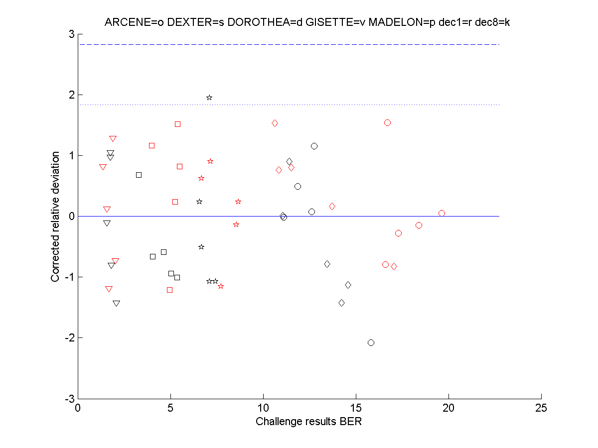
Second result verification. Fifty
submitted feature sets were tested to see whether their corresponding challenge
performance significantly differed from our reference classifier.
3) On-going work
We are presently working on reproducing the best challenge results with the simplest possible methods. Owing to the success of filter methods in this benchmark, we are conducting a systematic study, decoupling the problem of selecting features from that of classifying. We are testing classifiers including nearest neighbors, Parzen windows, SVMs, kernel ridge regression, tree classifiers, and neural networks, on the best feature subsets selected in the challenge. We are also generating feature subsets with various methods that we will test with our canonical classification methods. We are creating a library of routines that will be made publicly available.
The analysis of the challenge results also
revealed that hyperparameter selection may have played an important role
in
winning the challenge. Indeed, several
groups were using the same classifier (e.g. an SVM) and reported significantly
different results. We have started laying the basis of a new benchmark
on the theme of model selection and hyperparameter selection.