|
|
Causation and Prediction ChallengeAppendix A: Correlation analysis |
|
Further analysis of correlation between causation and prediction
The results of the causation and prediction challenge showed a poor correlation between the Fscore we had defined to assess causal feature relevance and the Tscore measuring prediction accuracy.We ended up creating a new Fscore, which correlates better with the Tscore. Consider the quatities called in information retrieval "precision" and "recall". The recall is the "sensitivity" (fraction of success of the positive class, i.e. the fraction of relevant features retrieved relatively to to the total number of relevant features). The precision is the fraction of relevant features in the features selected (i.e. 1-FDR, where FD is the "false discovery rate"). We found that both precision and recall correlate with Tscore, but precision correlates more. Recall is not a good metric for SIDO and CINA (real data + probes) because we must approximate the set of "relevant" features by the set of "true" features, among which some might be irrelevant. Conversely the fraction of true features in the set of features selected is a good proxi for the real precision, which cannot be computed directly. We also tried the Fmeasure=2*precision*recall/(precision+recall). Computing these scores required defining a set of good (relevant) features and a set of bad (irrelevant features). This is a difficult exercise sine all features have "some" degree of relevancy. To partially remedy that problem, we computed 3 versions of precision and recall, using as set of relevant features, set1="Markov blanket" or set2=MB+causes&effects or set3=all_relatives. The resulting scores is a weighted average using weights 3,2,1, to emphasize more the features, which should be more relevant. Based on such average precision and recall, we define the new Fscore as the precision for SIDO and CINA and the Fmeasure for REGED and MARTI.
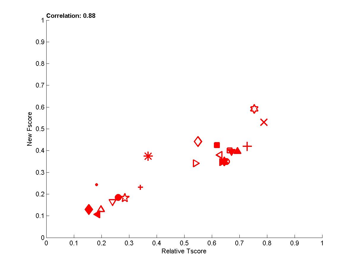
In the following plots, we show the new Fscore, as a function of Tscore. The horizontal line indicates the fraction of relevant features in the entire feature set. Hence, it can be seen that many entrants do better then selecting features at random since their feature set is significantly enriched in relevant features. The Tscore is normalized as follows: max(0, (Tscore-0.5)/(MaxTscore-0.5)) to indicate performance relative to the best achievable performance. Our observations include:
- We see that for test sets numbered 0, some of the top ranking entries have feature sets with precision no better than the entire feature set (some actually used the entire feature set). See for instance the entries of Gavin Cawley.
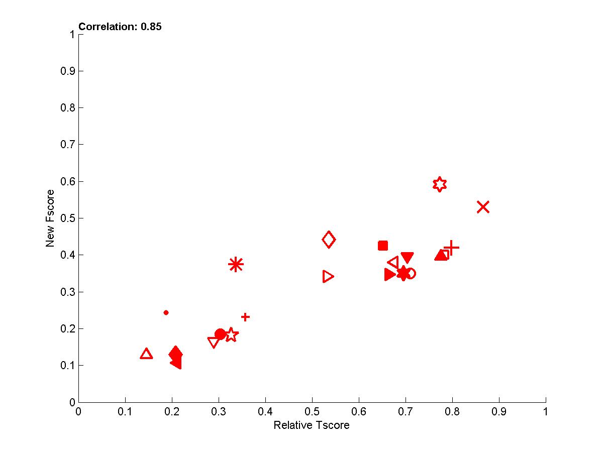
- Perhaps more surprisingly, some entries in for test sets 1 and 2 have poor Fscore and yet a good Tscore. This is particularly interesting because, in the case of test sets 0, the same irrelevant features are both in training and test data, so the classifiers can train to ignore them. For test sets 1 and 2, there are more irrelevant features in test data than in training data, due to the manipulations.
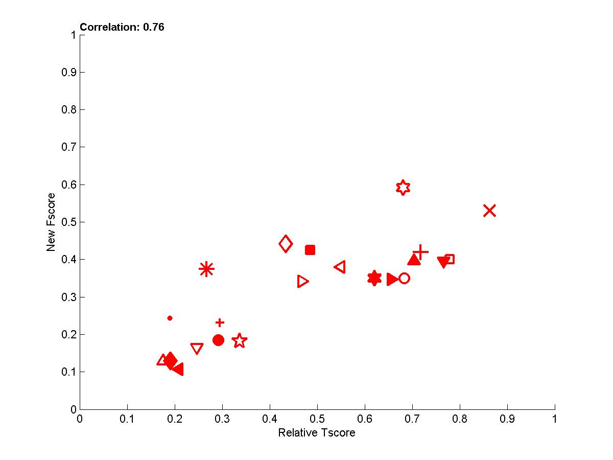
- The correlations for test sets 2 are more important than for test sets 1 because of their design. For REGED and MARTI, test set 1 has fewer members of the original Markov blanket that are manipulated then test set 2. For SIDO and CINA, all probes are manipulated, but the choice of values in test set 1 corresponds to a simle randomization, while in test set 2 the manipulations are made in an adversarial way to penalize more heavily people who select wrong features.
- Going back to the table of reference entries, we see that, if the Markov blanket (or the "manipulated" system) is known, using it gives an advantage. However finding it from training data is hard and training data must also be used to train the predictive model. As a result, the best performing entries often use many more features than the size of the Markov blanket, including a large number of relatives, partially compensating from erroneously selected irrelevant features.
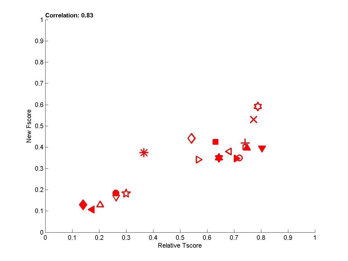
- To get rid of some of the variance, we averaged over several test sets the new Fscore and the Tscore to obtain the last plot, which demonstrates that there is overall good correlation between causation and prediction. We show below the whole table of corelation values between new Fscore and Tscore:
Set 0
Set 1
Set 2
Mean
REGED
0.34 ( 0.2)
0.10 ( 0.7)
0.65 (0.006)
0.58 ( 0.02)
SIDO
0.31 ( 0.2)
0.38 ( 0.2)
0.44 ( 0.1)
0.56 ( 0.01)
CINA
-0.30 ( 0.3)
-0.00 ( 1)
0.52 ( 0.05)
0.47 ( 0.05)
MARTI
0.66 ( 0.02)
0.94 (7e-006)
0.67 ( 0.02)
0.87 (0.0002)
Mean
0.90 (2e-008)
0.83 (2e-006)
0.76 (4e-005)
0.84 (2e-018)
Table A1 : Correlation between New Fscore and Tscore. The mean corresponds the the correlation of scores averaged over several datasets.
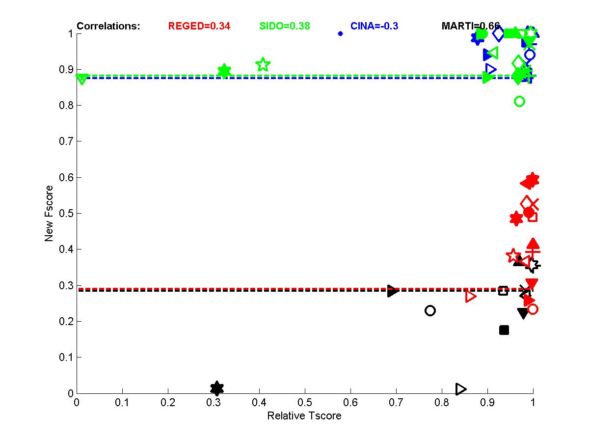
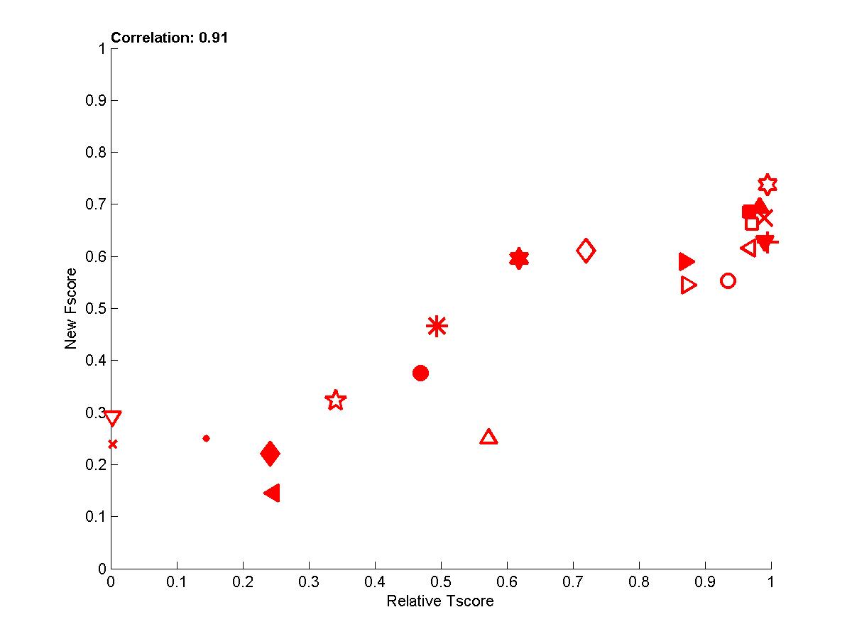
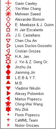
Figure A1: Test sets 0 -- New Fscore a function of relative Tscore. Right: results for all 4 tasks. Left results averaged over all 4 tasks.
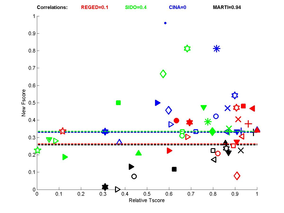
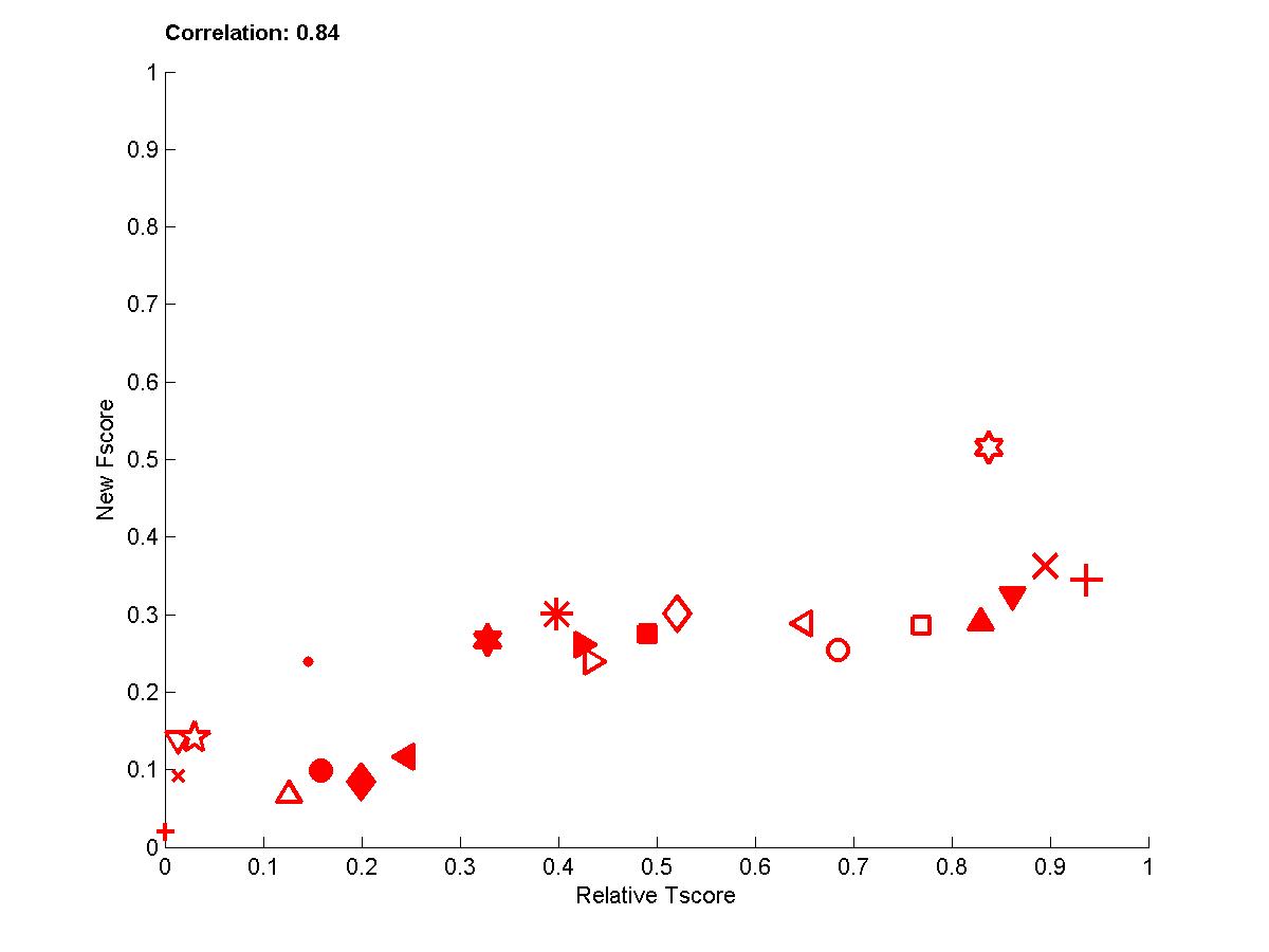
Figure A2: Test sets 1 -- New Fscore a function of relative Tscore. Right: results for all 4 tasks. Left results averaged over all 4 tasks.
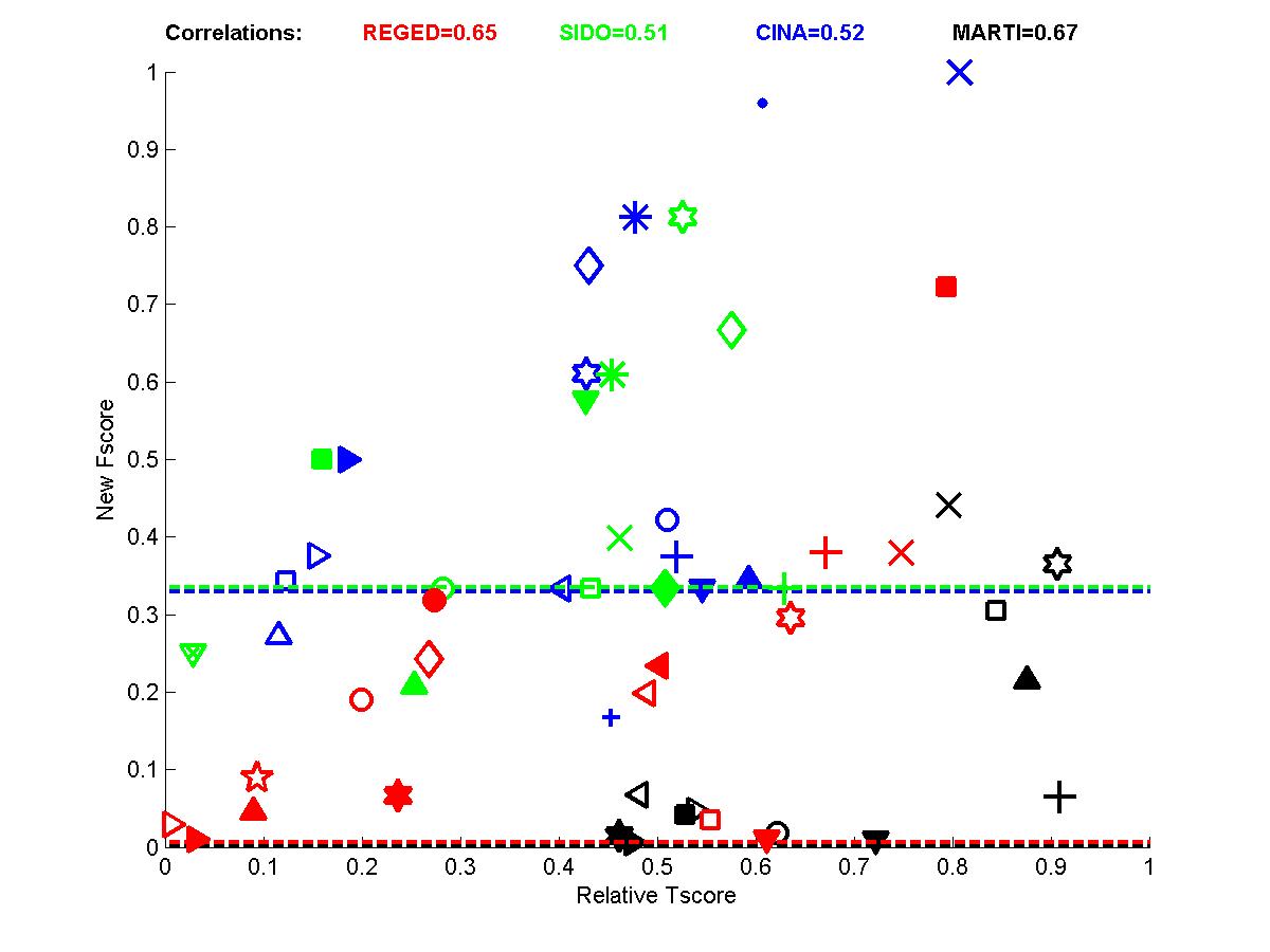
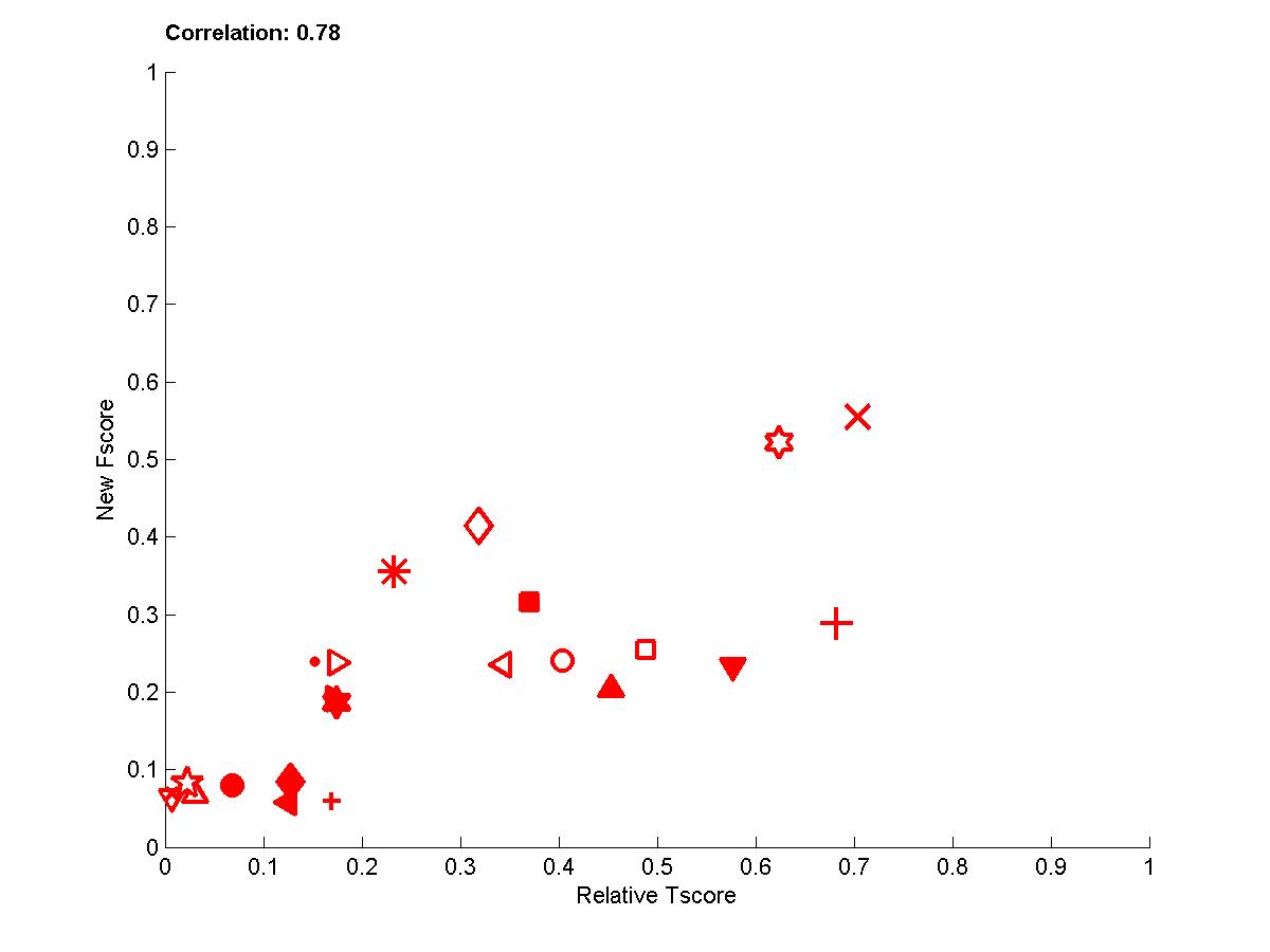
Figure A3: Test sets 2 -- New Fscore as a function of relative Tscore. Right: results for all 4 tasks. Left results averaged over all 4 tasks.
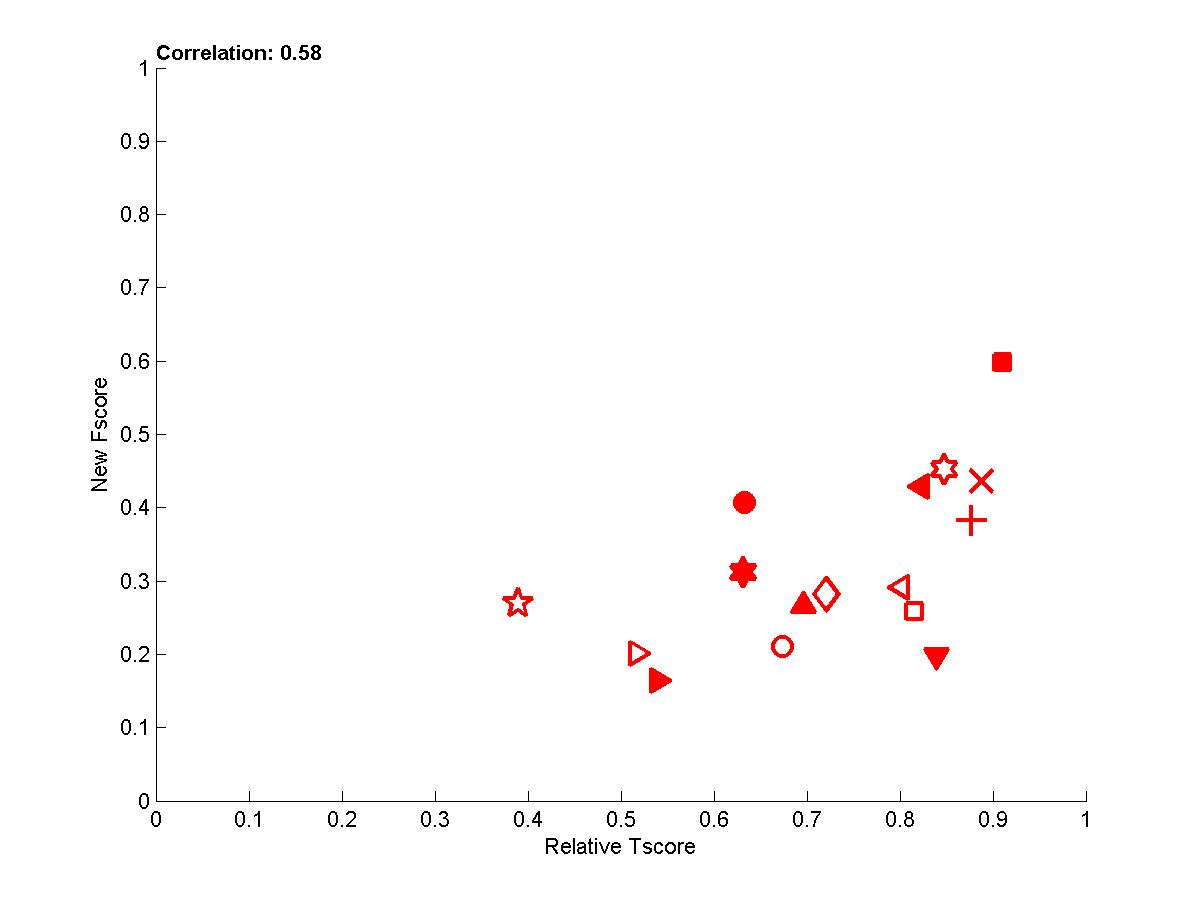


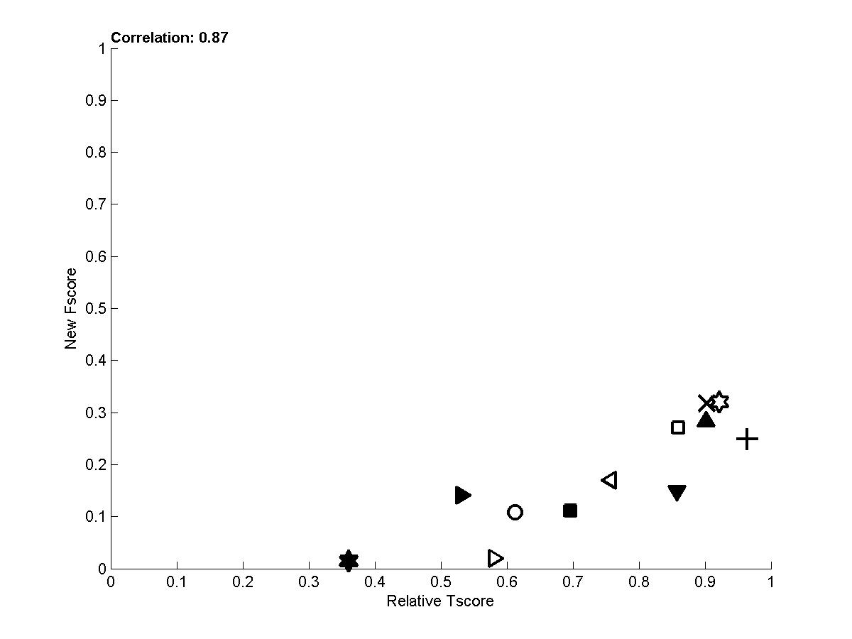
Figure A4: Results averaged over sets 0, 1, and 2 for the 4 tasks (red=REGED, green=SIDO, blue=CINA, black=MARTI).
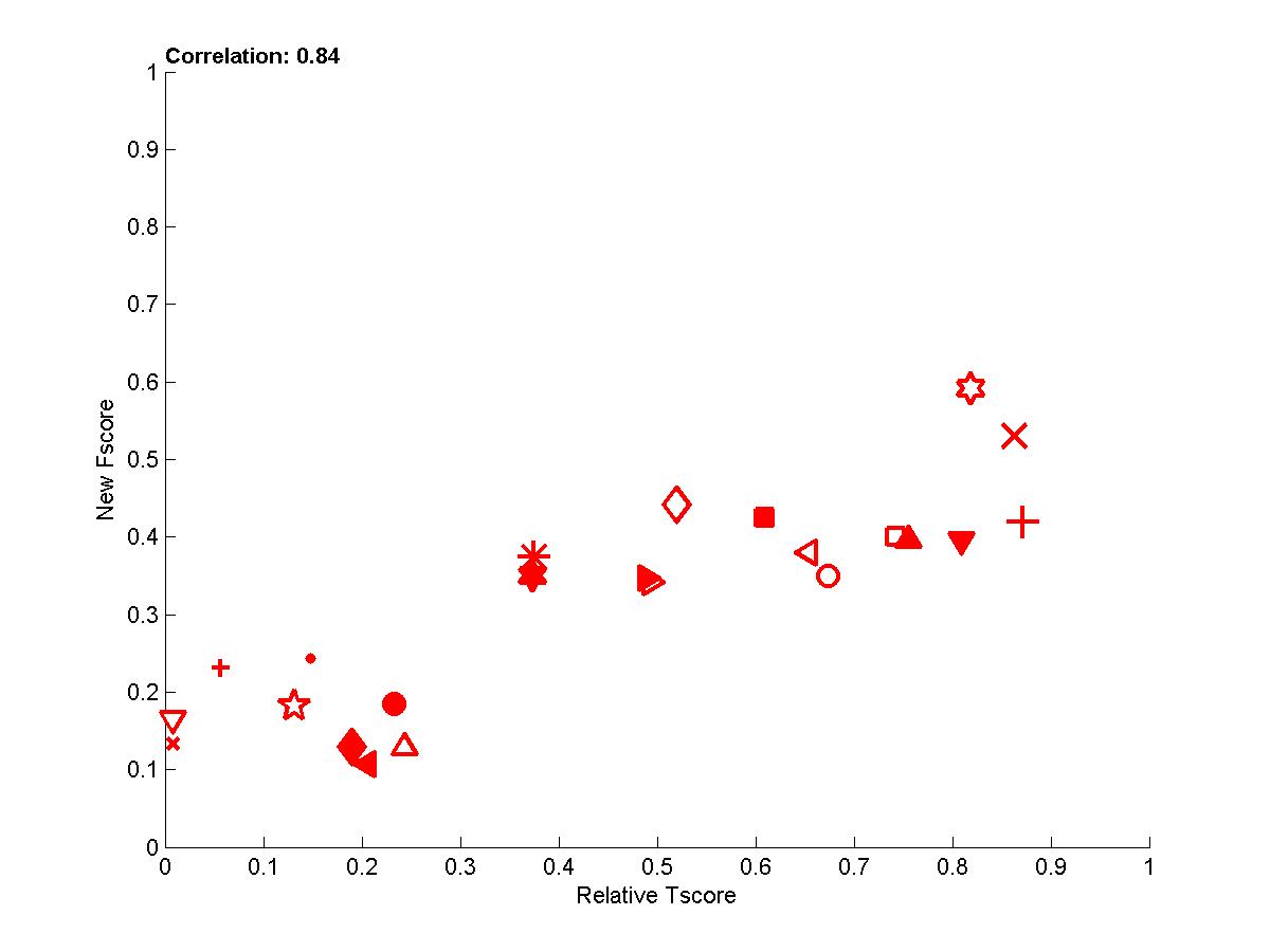
Figure A5: Average scores -- Performance of participants averaged over all datasets.