|
|
Causation and Prediction ChallengeAppendix B: Pairwise Comparisons |
|
Further analysis of participant performance: pairwise comparisons
The results of the causation and prediction challenge were biased in favor of people who returned tables of results. This section corrects for this bias by making pariwise comparisons of participant results at equal number of features.According to the rules of the challenge, people could return prediction results for nested subsets of features of size 1, 2, 4, 8, ... N. The best Tscore (test set AUC) of all these predictions was selected to rank their entries. We encouraged in this way people to perform feature ranking and return result tables, from which we could make graphs of performance as a function of the number of features.
By analyzing these graphs, we made the following observations:
- Optimal feature subsets larger than the Markov blanket: The best results were obtained often with large feature subsets, much larger than the Markov Blanket of the target for the manipulated test distribution, apparently because including (many) predictive features not belonging to the Markov Blanket helps compensating for wrongly included irrelevant features and wrongly discarted MB features.
- Causal relevance of features obtained with test set information: Selecting the results corresponding to the best Tscore was a means of selecting indirectly the subset with the best proportion of causally relevant features using information from test data. Hence even algorithm peforming no causal discovery at all obtained feature sets enriched in causally relevant features.
- Causal dsicovery and feature ranking: A majority of people from the feature selection community chose to return result tables while few people from the causal discovery commnity chose this option. This can be explained by the fact that many feature selection algorithms return feature rankings or nested subsets of features while causal discovery algorithms return single feature subsets (e.g. the Markov Blanket, or the sets of direct causes).
- Two participants with a single feature set: compare directly their predicition performance
- One participant with a single feature set of size F and one with results for nested subsets: compare the performances using F features (intepolating performances eventually for the person having provided results for the nested feature subsets)
- Two participants with nested feature subsets: compare the results for a number of features corresponding to the median of the number of features of participants having returned a single feature set.
Conclusion:
The correlations between Fscore and Tscore are enhanced considerably with this pairwise comparison (See table B1). The analysis of the graphs indicate that the team of Jianxin Yin and Prof. Geng did best both with respect to causal disovery and target prediction performance. However, Vladimir Nikulin and Marc Boullé closely match the prediction performances while using plain feature selection. By examining the entries made, it appears that Vladimir Nikulin may have been significantly influenced by the feed-back from the quartiles provided during the challenge. However, Marc Boullé made only one submission and uses methods making independence assumptions between features. Nonetheless, on REGED, the team of Laura Brown and Ioannins Tsamardinos (LEB&YT) comes ahead, and on SIDO and MARTI the team of Jianxin Yin and Prof. Geng comes ahead both with respect to Tscore and Fscore. It is only on CINA that the feature selection people get great prediction performance with no causal discovery.
Table B1: Correlation between Fscore and Tscore. We show the Pearson correlation coefficient and pvalue in parenthesis. All correlations outlined are significant with 95% confidence.
| |
Set 0 | Set 1 | Set 2 | Mean |
| REGED | 0.55 (0.007) | 0.55 (0.006) | 0.63 (0.001) | 0.62 (0.001) |
| SIDO | 0.36 ( 0.09) | 0.64 (0.001) | 0.60 (0.002) | 0.70 (0.0002) |
| CINA | 0.36 ( 0.09) | 0.69(0.0003) | 0.65 (0.0007) | 0.72 (0.0001) |
| MARTI | 0.94 (1e-11) | 0.96(1e-13) | 0.90 (4e-9) | 0.95 (2e-12) |
| Mean | 0.64 (0.001) | 0.75(3e-5) | 0.73 (7e-5) | 0.70 (3e-11) |
Warning: Our mehod of scoring introduced an undesirable bias. We recommend not to use the best of several performances using test data in a challenge in which test data is not drawn from te same distribution as the training data because this amounts to injecting important information on the test distribution in the results. This is very important in comparisons of causal discovery methods, if many methods are tried. If many methods are tried, because of variance in the results, some methods not performing causal dicovery may perform surprisingly well.
Figure B1: Performance of participants
for test sets 0. Left: for each dataset. Right: averaged over datasets.
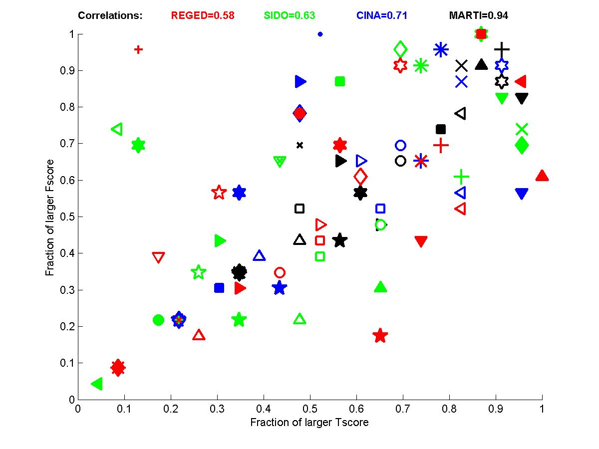

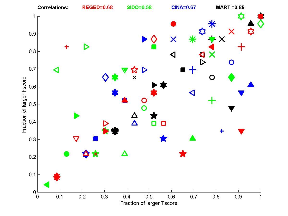
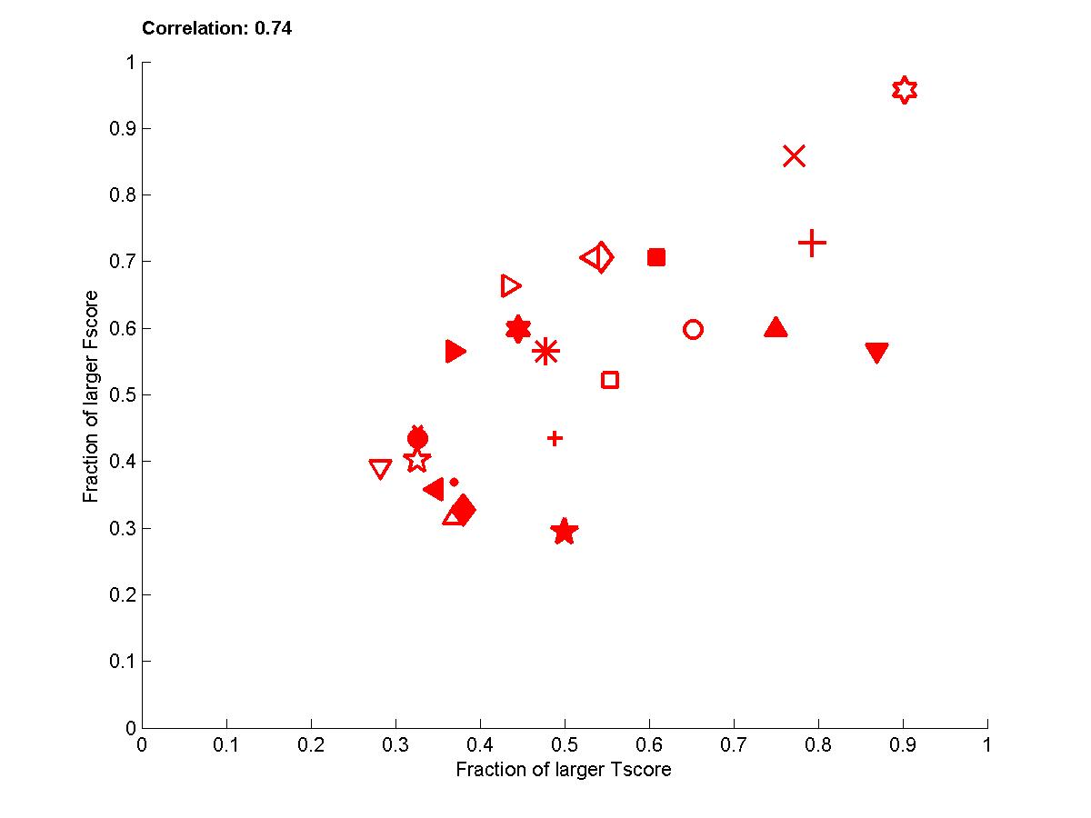
Figure B3: Performance of participants for test sets 2. Left: for each dataset. Right: averaged over datasets.
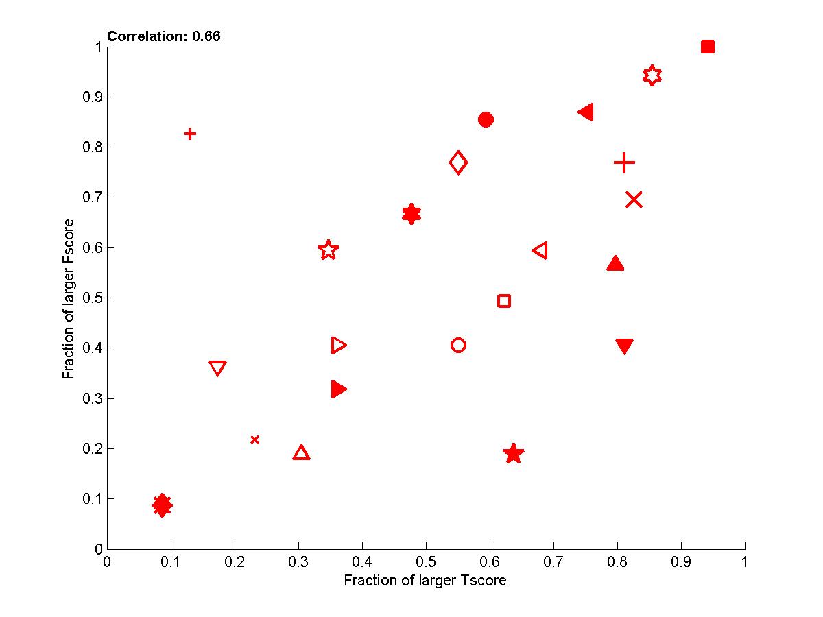
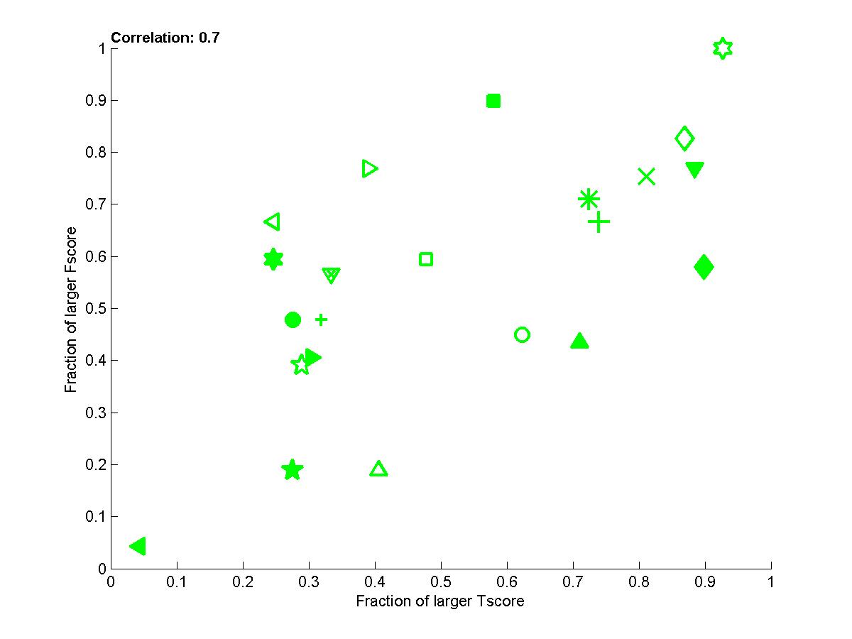
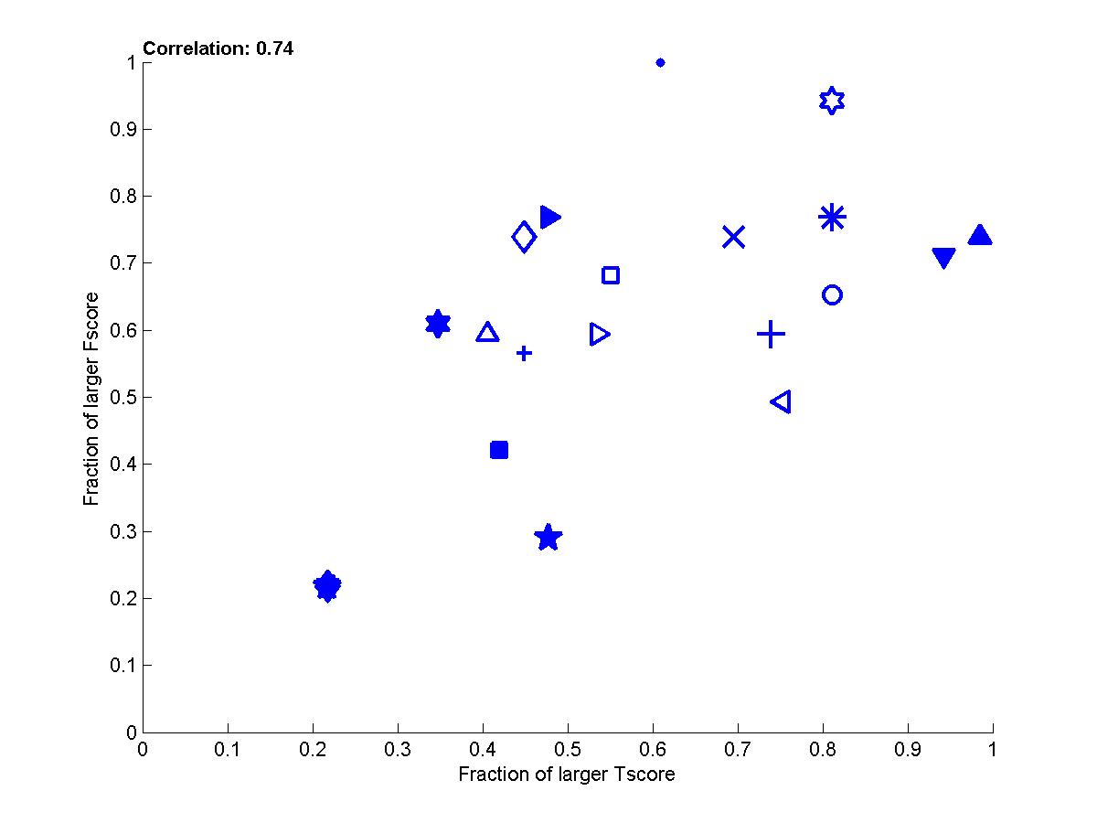

Figure B4: Performance of participants averaged
over sets 0,1, and 2 for the 4 tasks
(red=REGED, green=SIDO, blue=CINA, black=MARTI).
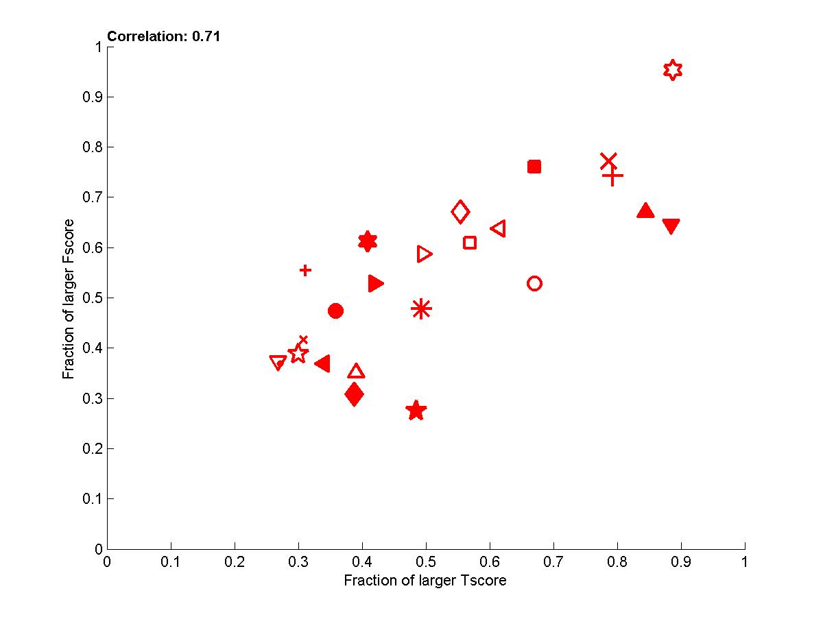
Figure B5: Performance of participants averaged over all sets 0,1, and 2 and all 4 tasks.
Figure B2: Performance of participants
for test sets 1. Left: for each dataset. Right: averaged over datasets.
Figure B3: Performance of participants for test sets 2. Left: for each dataset. Right: averaged over datasets.
(red=REGED, green=SIDO, blue=CINA, black=MARTI).
Figure B5: Performance of participants averaged over all sets 0,1, and 2 and all 4 tasks.