|
|
Causation and Prediction Challenge Analysis |
|
Summary:
The causation and prediction
challenge started on December 15, 2007 and ended on April 30,
2008. Four tasks were proposed from various application domains. Each
dataset included a training set drawn from a "natural" distribution
and 3 test sets: one from the same distribution as the training set (labeled
0) and 2 corresponding to data drawn when an external agent is manipulating
certain variables. The goal of the challenge was to predict as well
as possible a binary target variable, whose value on test data was withheld.
In addition, the participants were asked to provide the list of variables
(features) they used to make predictions. The tasks were designed such
that the knowledge of causal relationships between the predictive variables
and the target should be helpful to making predictions. Causation and
prediction are tied because manipulated variables, which are not direct
causes of the target, may be more harmful than useful to making predictions.
In the extreme case when all variables are manipulated, only the direct
causes are predictive of the target. The effectiveness of causal discovery
is assessed with a score, which measures how well the features selected
coincide with the Markov blanket of the target for test set distribution.
Part of our analysis is to observe under which condition this score is
correlated with prediction accuracy.
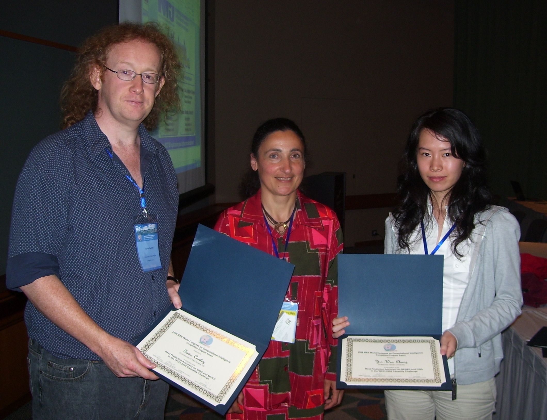
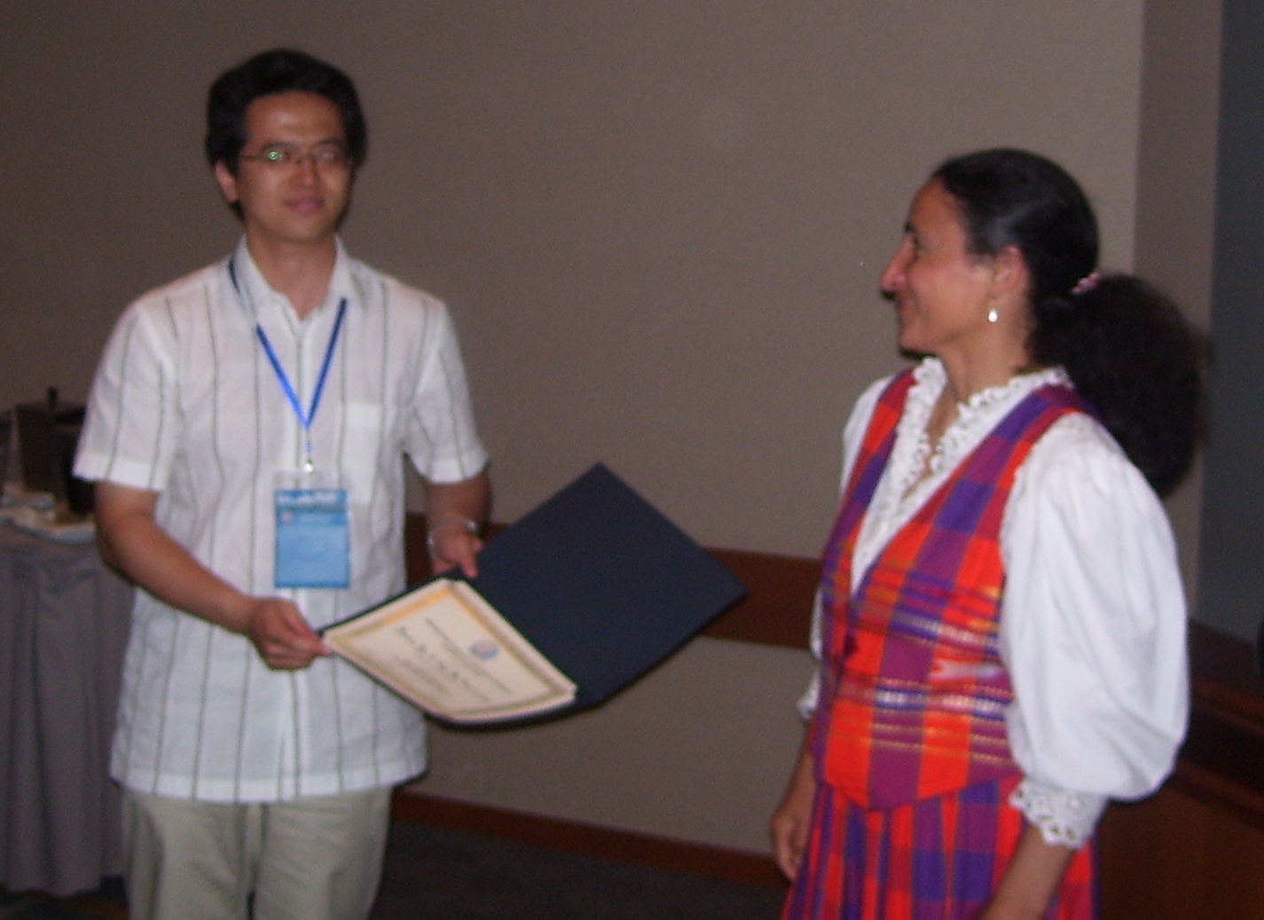
Left: Gavin Cawley and Yin-Wen Chang receiving their award from Isabelle Guyon. Right: Jianxin Yin receiving his award from Isabelle Guyon.
Publication:
- Design and Analysis of the Causation and Prediction Challenge
- Isabelle Guyon, Constantin Aliferis, Greg Cooper, André Elisseeff, Jean-Philippe Pellet, Peter Spirtes, and Alexander Statnikov; JMLR W&CP 3:1-33, 2008.
Winners:
Left: Gavin Cawley and Yin-Wen Chang receiving their award from Isabelle Guyon. Right: Jianxin Yin receiving his award from Isabelle Guyon.
- Gavin Cawley (University of East Anglia, UK): Best prediction accuracy on SIDO and MARTI, using Causal explorer + linear ridge regression ensembles. Prize: $400 donated by Microsoft.
- Yin Wen Chang (National Taiwan University): Best prediction accuracy on REGED and CINA, using SVM. Prize: $400 donated by Microsoft.
- Jianxin Yin and Prof. Zhi Geng’s group (Peking University, Beijing, China): Best overall contribution (best on Pareto front causation/prediction, new original causal discovery algorithm), using Partial Orientation and Local Structural Learning. Prize: free WCCI 2008 registration.
Description of the datasets:
We published a technical memorandum describing the datasets, how we created them, and some baseline results.The data are available from the website of the challenge, where each dataset is described. Briefly:
- REGED is a dataset generated
by a simulator of gene expression data, which was trained on
real DNA microarray data. The target variable is "lung cancer". Hence,
the task is to discover genes, which trigger disease or are a consequence
of disease. The manipulations simulate the effect of agents such as drugs.
For REGED1, the list of manipulated variable is provided, but not for
REGED2. REGED has 999 features, of which the Markov blanket contains 2
direct causes, 13 direct effects and 6 spouses in REGED0, but only 2 direct
causes, 6 direct effects and 4 spouses in REGED1, and 2 direct
causes in REGED2.
- SIDO consists of real data, from a drug discovery problem. The variables represent molecular descriptors of pharmaceutical compounds, whose activity on the HIV virus must be determined (the target variable). Knowing which molecule feature is a cause of activity would be of great help to chemical engineers to design new compounds. To test the efficacy of causal discovery algorithm, artificial "distractor" variables (called "probes") were added, which are "non-causes" of the target. All the probes are manipulated in the test sets SIDO1 and SIDO2. The probes must be filtered out to get a good causal discovery score and good prediction performance on test data. SIDO has 4932 features, of which 1644 real features and 3288 probes.
- CINA is also a real dataset. The problem is to predict the revenue level of people from census data (marital status, years of study, gender, etc.). As a causal discovery problem, the task is to find causes, which might influence revenue. Similarly as for SIDO, artificial variables (probes) were added. CINA has 132 features, of which 44 real features and 88 probes; all probes are manipulated in CINA1 and 2.
- MARTI is a noisy version of REGED. Correlated noise
was added to simulate measurement artifacts and introduce spurious
relationships between variables. This dataset illustrates that without
proper calibration/normalization of data, causal discovery algorithms
may yield wrong causal structures. MARTI has 1024 features and the same
causal graph as REGED. However, 25 calibrant variables were added to help
taking out the noise.
Reference entries:
We searched for the entries, which obtained best Tscore among all the Reference entries, which were made with the knowledge of the true Markov blanket (Fscore=1). With a few exceptions, the Tscore reached is not statistically significantly different from the best among all entries, regardless of Fscore (see this table). The interesting exceptions are for SIDO0 and CINA1 where the best Tscore is reached by entries having Fscore~0.5, showing the robustness of these classifiers to a large number of distractors. The SIDO0 entry uses linear ridge regression and the CINA1 entry uses naive Bayes.Learning Curves:
In Figure 1, we show the value of the best test set prediction score (Tscore) for predicting the target variable obtained by participants, as a function of number of days in the challenge. The Tscore used here is the area under the ROC curve. The datasets REGED and SIDO were introduced from the beginning of the challenge while CINA was introduced a month later and MARTI mid-way. We show as a thin line the performance level of the best Reference entry made by the organizers (using knowledge of causal relationships not available to the participants). We see that this value is closely reached by the participants by the end of the challenge for all 3 variant of REGED and MARTI whereas some improvement could still ne gained on SIDO1 and 2 and CINA1 and 2. Progresses are made by steps.
Figure 1: Leaning curves. The thin horizontal lines indicate
the best achievable performance, knowing the causal relationships (solid
line for set 0, dashed line for set 1, and dotted line for set 2.
Performance Histograms:
In Figure 2, the distribution of Tscores is represented by histograms of all the complete entries made throughout the challenge. The dashed vertical line represents the best Reference entry made by the organizers (using knowledge of causal relationships not available to the participants). The solid vertical line represents the best final entry made by the participants (only one final entry was allowed per participant). We note that the particpants did not always select their best entries as final submission, which indicates that the feed-back on performance they were getting on-line was not sufficient to perform model selection. Still, it may have biased the results, particularly on version 0 of the datasets, for which there is not a wide spread in results of the top ranking submissions. Hence, falling out of the top 25% was a strong indication of performance loss. We see that for the version 0 of the datasets, the Reference performances are reached. Hence, the on-line feed-back may have had the effect of pumping performance up. However, version 0 is the only one in which training data and test data have the same distribution. Hence cross-validation gives a very strong feed-back. Additionally, many more featurs are predictive in version 0 since, due to manipulations, a lot of features are made irrelevant in versions 1 and 2. We see no indication that "pumping" ocurred for versions 1 and 2. To further detect any potential "pumping" effect, we analyzed the progress of individual participants (see individual results). We notice that for version 0, the top 2 quatiles are very close to one another. Towards the end of the challenge, the entries oscillate over and under the top quartile line, giving very strong feed-back to the participants. Also, as the number of entries grow, the top quartile values are drifting up, so participants having entered late in the game did not succeed in catching up and benefit from this feed-back.
Figure 2: Histograms of Tscores.
Analysis of results by dataset:
In Figures 3, 4, 5, 6, we show the individual participant results for their last complete entry. The entrants who qualified for the final ranking (i.e., having a complete entry, disclosing their name, providing their feature set, providing a fact sheet, and cooperating with verification tests) have their rank indicated in parenthesis. We also show on the graph the last complete entry of participants, who did not comply with all the requirements or did not compete towards the prizes for other reasons (there are referred to by they psudonym of initials). According to the instructions, the participants could provide sorted or unsorted lists of features. Participants having supplied a sorted list of features have one star after their name. They also had the option of varying the number of features used, following nested subsets of features derived from their ranking. The participants who supplied a table of results corresponding to using nested subsets of features have 2 stars after their name.We show 3 graphs:
- Tscore: The test set AUC for the prediction of the target variable.
- Fscore: The AUC for the prediction of which features belong to the Markov blanket.
- Fnum: The number of features used.
We observe some correlation between Fscore and Tscore, but some notable exceptions:
- Some participants provided an unsorted list of all features or no list at all. They get an Fscore of 0.5. This does not necessarily indicate that they performed no feature selection: Some ensemble methods use multiple feature subsets and we did not have provisions in our format for reporting such cases.
- Some participants performed good causal discovery (high Fscore) but did not get good prediction performance (low Tscore). This could be attributed to a bad classification algorithm and needs to be further investigated case by case. For REGED2, for instance, many people discovered the causes of the target exactly. Yet, they do not necessarily predict well the target
- The Fscore gives equal importance to good features
rightly selected and bad features rightly discarded. Hence for REGED2
where there are very few good features, most people who got them all
get a very high Fscore. The proportion of good features in the selected
feature set (so-called "precision") correlates a little better with Tscore,
particularly when the good feature set is taken as all relatives instead
of just Markov blanket members.
- Interestingly, some participants obtained good Tscore for a very bad Fscore. For the test sets labeled 0, this is not surprising since using all the features often yields better performance than using features selection: generally most good regularized classifiers are robust against the presence of irrelevant features. For the test sets labeled 1 and 2, some manipulated variables should introduce a significant disturbance, which should give an advantage to people who got rid of them.
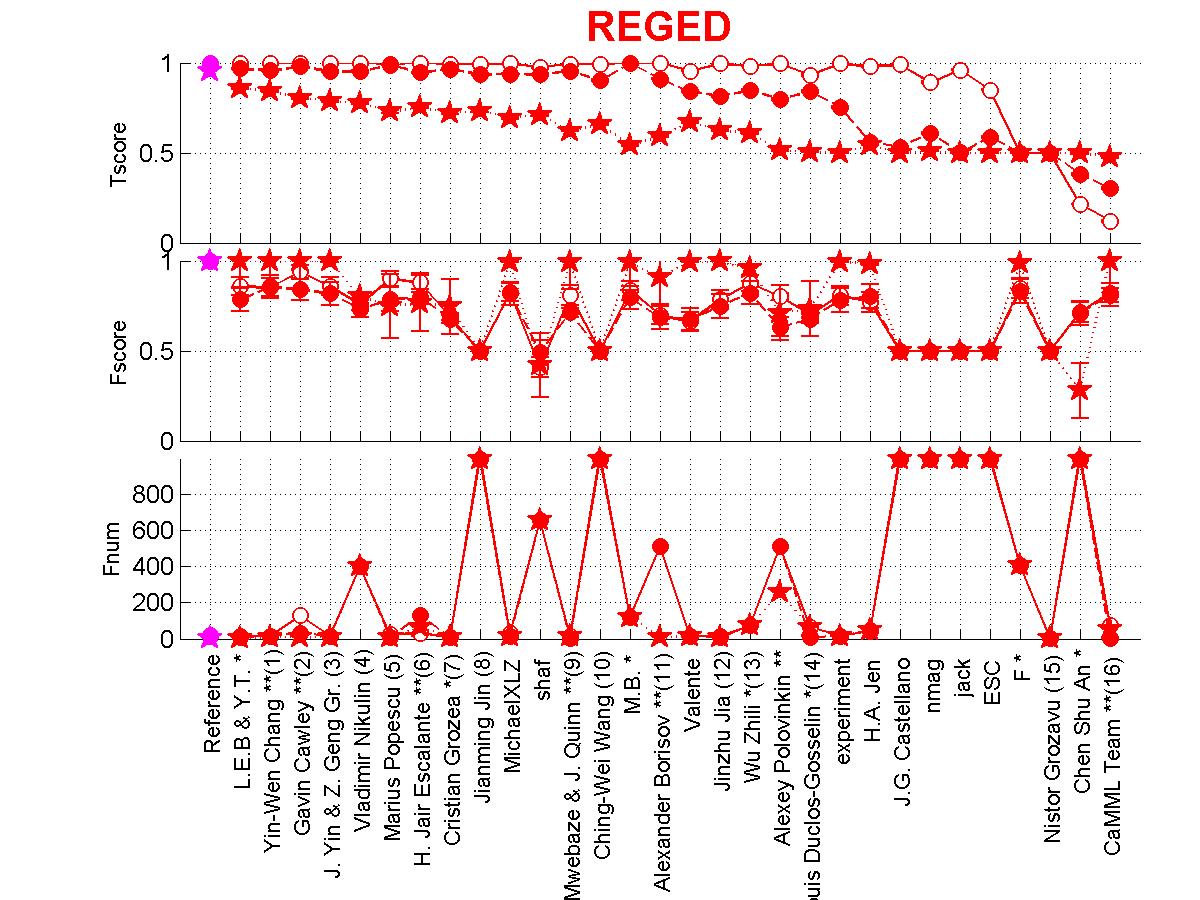
Figure 3: Scores of participants for REGED. Circle=REGED0,
Full circle=REGED1, Star=REGED2.
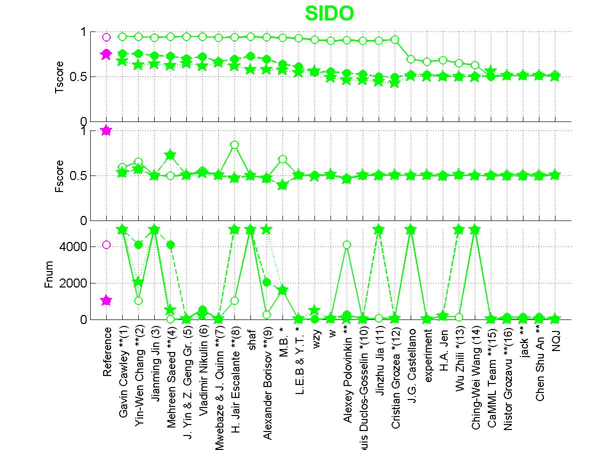
Figure 4: Scores of participants for SIDO. Circle=SIDO0, Full circle=SIDO1, Star=SIDO2.
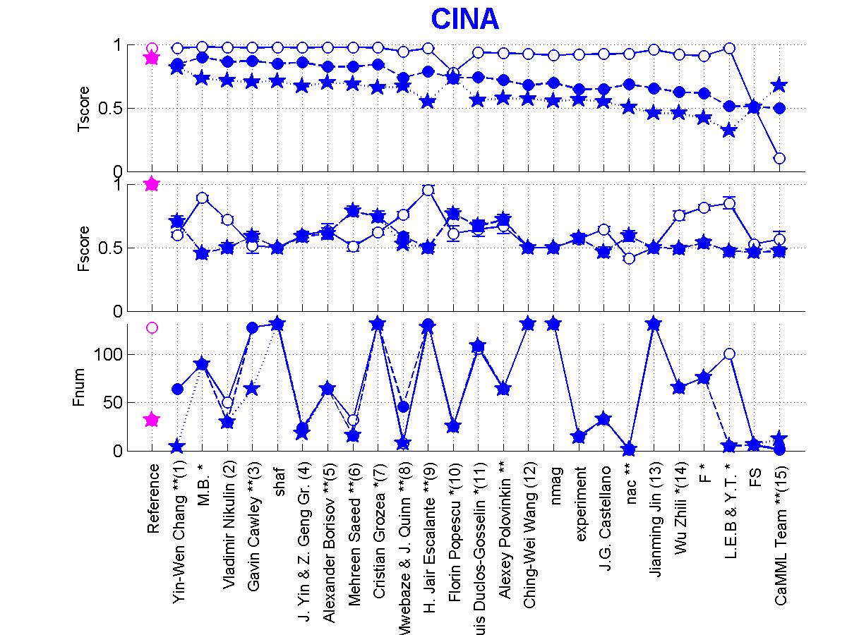
Figure 5: Scores of participants for CINA. Circle=CINA0, Full circle=CINA1, Star=CINA2.

Figure 6: Scores of participants for MARTI. Circle=MARTI0, Full circle=MARTI1, Star=MARTI2.
Figure 4: Scores of participants for SIDO. Circle=SIDO0, Full circle=SIDO1, Star=SIDO2.
Figure 5: Scores of participants for CINA. Circle=CINA0, Full circle=CINA1, Star=CINA2.
Figure 6: Scores of participants for MARTI. Circle=MARTI0, Full circle=MARTI1, Star=MARTI2.
Further analysis of correlation between causation and prediction
These results prompted us to investigate the correlation between Tscore and various measures evaluating the feature set to see whether a better correlation between causation and prediction could be obtained.We provide a detailed analysis and many more graphs in Appendix A:
We ended up creating a new Fscore, which correlates better with the Tscore, based on the information retrieval notions of precision and recall. We define a precision, which assesses the fraction of causally relevant features in the feature set selected (precision=num_good_selected/num_selected) and a recall, which measures the fraction of all causally relevant features retrived (recall=num_good_selected/num_good). For REGED and MARTI, the new Fscore is the Fmeasure=2*precision*recall/(precision+recall), while for the datasets SIDO and CINA we simply use the precision (because recall is not a meaning ful quantity for real data with probes since we do not know which variables are relevant). This new Fscore correlates well with Tscore, as shown in Figure 7.
In addition, in Appendix B, we performed another analysis, which aims at correcting the bias introduced by picking up the best performance on the test set for people who returned a series of predictions on nested subsets of features. We performed paired comparisons for identical feature numbers. In Figure 8, we show how this affect performances.
Finally, we are presently conducting complementary experiments to factor out the influence of the classifier, by training the same classifiers on the feature sets of the participants.
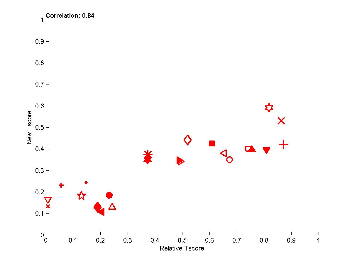
Figure 7: Performance of participants averaged over all datasets (all 4 tasks and all test set versions).
The new Fscore is plotted as a function of the relative Tscore: (Tscore-0.5)/(MaxTscore-0.5).
Figure 8: Performance of participants averaged over all datasets (all 4 tasks and all test set versions).
Here we show the fraction of times one participant is better than another one in pairwise comparisons for identical numbers of features.
Individual participant results:
(including graphs and fact sheets)Chen Chu An
Alexander Borisov
M.B.
L.E.B & Y.T.
CaMML Team
J.G. Castellano
Gavin Cawley
Yin-Wen Chang
Louis Duclos-Gosselin
H. Jair Escalante
Cristian Grozea
Nistor Grozavu
Jinzhu Jia
Jianming Jin
H.A. Jen
E. Mwebaze & J. Quinn
Vladimir Nikulin
Alexey Polovinkin
Florin Popescu
Marius Popescu
Mehreen Saeed
J. Yin & Z. Geng Gr.
Ching-Wei Wang
Wu Zhili
Full Result Tables:
Tables of results are available in HTML format and text format. In addition we provide tables of ranked results.Verifications: Letter sent to top entrants
As one of the top ranking participants, you will
have to cooperate with the organizers to reproduce your results
in order to qualify for the prizes. The outcome of the tests (or
the absence of tests) will be published. To that end, we expect
you to:1) Elaborate on your method in the fact sheet:
- What specific feature selection methods did you try?
- What else did you try besides the method you submitted last? What do you think was a critical element of success compared to other things you tried?
- In what do the models for the versions 0, 1, and 2 of the various tasks differ?
- Did you rely on the quartile information available on the web site for model selection or did you use another scheme?
- In the result table you submitted, did you use nested subsets of features from the slist you submitted?
- Did you use any knowledge derived from the test set to make your submissions, including simple statistics and visual examination of the data?
2) Upload by May 15 your code to:
cp.clopinet.com
login: ywc
password: yinwen4wcci (change your password)
Go to "All files" an click "upload file"
** IMPORTANT: the code should be strictly standalone respect the following guidelines:
- Provide both executables (Windows and/or Linux) and source code for TWO SEPARATE training and test modules, called yourname_train and yourname_test.
- The two modules should be stricly standalone and include all necessary libraries compiled in and have no command line arguments.
- The modules should regularly output to STDOUT a status of progress.
- The modules should regularly save partial results so if they need to be interrupted, they can be restarted from intermediate results.
- The two modules will read and write to disk files including:
* a configuration file "config.txt" including the path to directories DATA_DIR where data are, MODEL_DIR where the models are, and OUTPUT_DIR where outputs should be written
* the data in the challenge standard formats to be read from DATA_DIR
* files "dataname[num]_manip.txt" specifying which features are manipulated in the test data to be read from DATA_DIR
* a file "marti0_calib.txt", special for MARTI, containing the calibrant numbers
* the models in a format you can freely choose to be written to MODEL_DIR
* the prediction results (including feature lists and output predictions) in the same format as challenge submissions to be written to OUTPUT_DIR
A) The training program will:
- Read from the current directory the configuration file "config.txt", indicating DATA_DIR and MODEL_DIR (keyword followed by path name, separated by newline)
- Read from DATA_DIR the training data (in standard format; since all 3 training sets are the same for a given task, we will use only version 0; only data from one task will be present in DATA_DIR) and the files "dataname[num]_manip.txt" indicating the list of manipulated variables, see self explanatory format attached.
- Produce models for test sets 0, 1, and 2 saved in OUTPUT_DIR
To save time, since much of the training may be similar for the versions 0, 1, and 2, the training module should process everything at once and output models for all 3 versions. The training module should save feature sets or feature rankings in MODEL_DIR. If nested subsets of features are used, the training module should produce models for all subsets. Therefore, it is important that the module can be restarted if it gets interrupted and all intermediate results be stored.
B) The test program will:
- Read from the current directory the configuration file "config.txt", indicating DATA_DIR, MODEL_DIR, and OUTPUT_DIR (keyword followed by path name, separated by newline)
- Read the test data from DATA_DIR (in standard format). Test sets for all 3 versions of a given task will be found in that directory and should all be processed.
- Load the corresponding model(s) from MODEL_DIR
- Output the submission as it was made to the website in OUTPUT_DIR
Special Matlab instructions:
- Provide 2 Matlab functionsA) [yourname]_train(data_name, train_data_dir, model_dir, log_dir)
This function should read from train_data_dir
* [data_name]_train.data
* [data_name]_train.targets
* [data_name]_manip.txt
and should output models to model_dir. Optionally, log_dir can be used to log messages about the status/completion of learning.
B) [yourname]_test(data_name, test_data_dir, model_dir, output_dir)
This function should read from test_data_dir
* [data_name]_test.data
and reload models from model_dir. Then it should produce predictions to output_dir.
- We will run your code of the original datasets and variants.
- Do not pass the full dataset archive as an argument to the program, pass a directory name.
- train_data_dir and test_data_dir will be 2 separate directories to make sure we do not load accidentally test data during training.